SIMULATION OF EXTRA HIGH VOLTAGE LONG TRANSMISSION LINES

SIMULATION OF EXTRA HIGH VOLTAGE LONG TRANSMISSION LINES

ABSTRACT

The electrical power system mainly consists of three principle divisions the generating stations, y he transmission system and the distribution system. The transmission lines are the connecting links between generating station and the distribution system and lead to other power system interconnections. Now a day, we are using Extra High Voltage (EHV) transmission lines for transmission of power between the generating station and distribution system .The main reasons behind it are the construction of super power stations of very large capacities necessities the transmission at high voltage for this we use EHV lines.At high voltages power loss is also reduced because losses are directly proportional to the square of current. The simulation of transmission line using MATLAB helps us to analyze the behaviors and parameters of transmission line under actual conditions. We are simulating a long transmission line and analyze the waveforms at sending and receiving end. The results obtained after simulation are used in the designing of Extra High Voltage Long Transmission Line Model.

INTRODUCTION

Electrical energy is generated in large hydro electric, thermal and nuclear super and super critical power stations these stations are generally situated far away from the load centers. This necessitates an extensive power supply network between the generating station and consumer load. This network may be divided into two parts transmission and distribution the main part of this transmission system. Transmission line transmits bulk electrical power from sending end to receiving end stations without supplying any consumer en route and it can be divided into two parts primary and secondary. The transmission voltage is re 66kV, 110kV, 132kV, 220kV, 400kV and 765kV.

The more the voltages of transmission line the better the performance and efficiency of the system. For this we use high voltage and extra high voltage transmission lines to transmit electrical power from the sending end substations to the receiving end substations. At the receiving end substations the voltage is stepped down to a lower value of 66kV, 33kv or 11kV. The secondary transmission system forms the link between the main receiving end substations and secondary substations. In the transmission line the voltage can vary as much as 10% or even 15% DUE TO variation in loads the transmission line is the main energy corridor in a power system. The performance of a power system is mainly dependent on the performance of the transmission lines in the system. It is necessary to calculate the voltage current and power at any point on the transmission line provided the values at one point are known. We are aware that in 3 phase circuit problem it is sufficient to compute results in one phase and subsequently predict results in the other 2 phases by exploiting the three phase symmetry. Although the lines are not spaces equilaterally and not transposed the resulting asymmetry is slight and the phases are considered to be balanced as such transmission line calculations are also carried out on per phase basis.

The transmission line performance is governed by its four parameters

Series resistance

Series inductance

Shunt capacitance

Shunt conductance

All these parameters are distributed over the length of the line. The insulation of a line us seldom perfect and leakage currents flow over the surface of insulators especially during bad weather this leakage is simulated by shunt conductance. The shunt conductance is in parallel with the system capacitance. Generally the leakage currents are small and the shunt conductance is ignored in calculations.

The transmission line may be classified as short, medium and long. When the length of the line is less than about 80km the effect of shunt capacitance can be ignored and the line is designated as a short line. When the length is between 80 and 250km the shunt capacitance can be considered as lumped and the line is termed as medium length line. Lines more than 250km long require calculation in terms of distributed parameters are knows as ling lines.

Two Port Networks

A pair of terminals at which a signal (voltage or current) may enter or leave is called a port. A network having only one such pair of terminals is called a one port network.

 

Figure 1. Two-port network

A two-port network (or four-terminal network, or quadripole) is an electrical circuit or device with two pairs of terminals. Examples include transistors, filters and matching networks. The analysis of two-port networks was pioneered in the 1920s by Franz Breisig, a German mathematician.

A two-port network basically consists in isolating either a complete circuit or part of it and finding its characteristic parameters. Once this is done, the isolated part of the circuit becomes a "black box" with a set of distinctive properties, enabling us to abstract away its specific physical buildup, thus simplifying analysis. Any circuit can be transformed into a two-port network provided that it does not contain an independent source.

A two-port network is represented by four external variables: voltage and current at the input port, and voltage and current at the output port, so that the two-port network can be treated as a black box modeled by the relationships between the four variables Vs, Is, Vr and Ir. There exist six different ways to describe the relationships between these variables, depending on which two of the four variables are given, while the other two can always be derived.

Note: All voltages and currents below are complex variables and represented by phasors containing both magnitude and phase angle.

The parameters used in order to describe a two-port network are the following: Z, Y, A, h and g. They are usually expressed in matrix notation and they establish relations between the following parameters:

(1)Input voltage V1

(2) Output voltage V2

(3) Input current I1

(4) Output current I2

ABCD Parameters

 

Figure 2.transmission network

Two port representation of a transmission network.

Consider the power system shown above. In this the sending and receiving end voltages are denoted by VS and VR respectively. Also the currents IS and IR are entering and leaving the network respectively. The sending end voltage and current are then defined in terms of the ABCD parameters as

So,

This implies that A is the ratio of sending end voltage to the open circuit receiving end voltage. This quantity is dimension less. Similarly,

 

i.e., B , given in Ohm, is the ratio of sending end voltage and short circuit receiving end current. In a similar way we can also define

 

Also,

The parameter D is dimension less.

Note: Here A and D are dimensionless coefficients, B is impedance andC is admittance. A negative sign is added to the output current I2in the model, so that the direction of the current is out-ward, for easy analysis of a cascade of multiple network models.

SIMULATION

Various blocks used

Resistor

The Resistor block models a linear resistor, described with the following equation:

Where,

V Voltage

I Current

R Resistance

Connections + and – are conserving electrical ports corresponding to the positive and negative terminals of the resistor, respectively. By convention, the voltage across the resistor is given by V(+) – V(–), and the sign of the current is positive when flowing through the device from the positive to the negative terminal. This convention ensures that the power absorbed by a resistor is always positive.

Capacitor

The Capacitor block models a linear capacitor, described with the following equation:

Where,

I Current

V Voltage

C Capacitance

t Time

Inductor

The Inductor block models a linear inductor, described with the following equation:

Where,

I Current

V Voltage

L Inductance

t Time

Voltage Sensor

The Voltage Sensor block represents an ideal voltage sensor, that is, a device that converts voltage measured between two points of an electrical circuit into a physical signal proportional to the voltage.

Voltage Measurement

The Voltage Measurement block measures the instantaneous voltage between two electric nodes. The output provides a Simulink signal that can be used by other Simulink blocks.

AC Voltage Source

The AC Voltage Source block implements an ideal AC voltage source. The generated voltage is described by the following relationship:

Negative values are allowed for amplitude and phase. A frequency of 0 and phase equal to 90 degrees specify a DC voltage source. Negative frequency is not allowed; otherwise the software signals an error, and the block displays a question mark in the block icon.

Scope

The Scope block displays its input with respect to simulation time.

The Scope block can have multiple axes (one per port) and all axes have a common time range with independent y-axes. The Scope block allows you to adjust the amount of time and the range of input values displayed. You can move and resize the Scope window and you can modify the Scope's parameter values during the simulation.

Solver Configuration

Each physical device represented by a connected Simscap block diagram requires global environment information for simulation. The Solver Configuration block specifies this global information and provides parameters for the solver that your model needs before you can begin simulation.

Each topologically distinct Simscape block diagram requires exactly one Solver Configuration block to be connected to it.

Breaker

The Breaker block implements a circuit breaker where the opening and closing times can be controlled either from an external Simulink signal (external control mode), or from an internal control timer (internal control mode).

Ground

The Ground block implements a connection to the ground.

Add

The Add block performs addition or subtraction on its inputs. This block can add or subtract scalar, vector, or matrix inputs. It can also collapse the elements of a signal.

Sine Wave

The Sine Wave block provides a sinusoid. The block can operate in either time-based or sample-based mode.

Fcn Block

The Fcn block applies the specified mathematical expression to its input. The expression can be made up of one or more of these components:

• u - The input to the block. If u is a vector, u(i) represents the ith element of the vector; u(1) or u alone represents the first element.
• numeric constants
• Arithmetic operators (+ - * /^)
• Relational operators (== != ><>= <=) — The expression returns 1 if the relation is true; otherwise, it returns 0.
• Logical operators (&& || !)-The expression returns 1 if the relation is true; otherwise, it returns 0.
• Parentheses
• Mathematical functions — abs, cos, sin, exp, log, pow, tan, sinh, sqrt etc.
• Workspace variables — Variable names that are not recognized in the preceding list of items are passed to MATLAB for evaluation.

PI Section Line

The PI Section Line block implements a single-phase transmission line with parameters lumped in PI sections. For a transmission line, the resistance, inductance, and capacitance are uniformly distributed along the line. An approximate model of the distributed parameter line is obtained by cascading several identical PI sections, as shown in the following figure.

Unlike the Distributed Parameter Line block, which has an infinite number of states, the PI section linear model has a finite number of states that permit you to compute a linear state-space model. The number of sections to be used depends on the frequency range to be represented.

PS Simulink Converter

The PS-Simulink Converter block converts a physical signal into a Simulink output signal. Use this block to connect outputs of a Physical Network diagram to Simulink scopes or other Simulink blocks.

The Output signal unit parameter lets you specify the desired units for the output signal. These units must be commensurate with the units of the input physical signal coming into the block. The Simulink output signal is unitless, but if you specify a desired output unit, the block applies a gain equal to the conversion factor before outputting the Simulink signal. For example, if the input physical signal coming into the block is displacement, in meters, and you set Output signal unit to mm, the block multiplies the value of the input signal by 10e3 before outputting it.

Display

The Display block shows the value of its input on its icon. You control the display format using the Format parameter:

• short - displays a 5-digit scaled value with fixed decimal point
• long - displays a 15-digit scaled value with fixed decimal point
• short_e - displays a 5-digit value with a floating decimal point
• long_e - displays a 16-digit value with a floating decimal point
• bank - displays a value in fixed dollars and cents format (but with no $ or commas)
• hex (Stored Integer) - displays the stored integer value of a fixed-point input in hexadecimal format
• binary (Stored Integer) - displays the stored integer value of a fixed-point input in binary format
• decimal (Stored Integer) - displays the stored integer value of a fixed-point input in decimal format
• octal (Stored Integer) - displays the stored integer value of a fixed-point input in octal format

First Simulation Model

In this we tried to implement the simulation of the transmission line by using its equivalent diagram.

 

Figure 3.first simulation model

Although there were no errors but the simulation was not showing desired results. There was also no consideration of length and solver configuration block was not implemented correctly.

Second Simulation Model

Consider the standard model1 of a transmission line (Fig. 4).

 

Figure 4. standard model of transmission line

Both the voltages and the currents can be separately analyzed using Kirchhoff‘s laws and put in terms that can be analyzed using Simulink. Let’s analyze the model, writing all time-based variable sin the transmission line in terms of the Laplace transform variable, s. The spatial variation of the transmission line will be in corporated into the discrete section number:

For the simulation of the voltage response of the transmission line, the voltageV1 across the capacitor in the first loop (which includes the voltage source in Fig.4) can be written in terms of the voltage source, Vs, and the voltage in the second loop V2 as

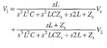(1) 

Where, Zsis the source impedance. In the transmission line, the elements L and C are the inductance per unit length, and the capacitance per unit length, respectively. The voltage across the capacitor in an Intermediate loop, n, can be written in terms of the similar voltage Vn-1 in the previous loop (n-l), and the voltage Vn+1 in the following loop (n+1).

(2)

A load impedance, ZL, is in parallel with the capacitor in the final loop, k. The load impedance can be linear or nonlinear.

We define the current in the load impedance at the end node, k, via the relation

(3)

Where g( Vk) is an arbitrary nonlinear function that has to be specified by the simulator. In the linear case, g(Vk) is equal to a constant multiplied by V(Fig. 5). From Fig. 5, we find the voltage Vk to be

(4)

 

Figure 5.simulink simulation of the voltage response of the transmission line

For purposes of simulating the current response of the transmission line, the current in the first loop (which includes the voltage source in Fig. 4) can be written in terms of the voltage source V, and the current in the second loop i2.

(5)

The current in an intermediate loop, n can be written in terms of the current in the previous loop (n-1) and the following loop (n+1):

(6)

For the case of linear load impedance, i =V/ZL, the load impedance ZL is in parallel with the capacitor in the final loop, k. The current in this loop is written in terms of the current in the previous loop (k-1)

(7)

Equations 5-7 determine the elements of a second transmission line. In Fig, 5, the critical Simulink elements are shown for the elements specified with Equations 1-4. A dialog menu with Simulink allows all parameters of the polynomial to be specified. We specify the voltage source, Vs, as a half sine wave generator, which acts as a pulse generator in the simulation. The amplitude and width were controllable parameters. In our application, fifteen identical intermediate elements were used. Although we will use only a Limited number of sections in our transmission line model, it can be generalized to include as many as desired.

In addition, the user can specify numerical values for the circuit elements L, C, Zs, and ZL. For clarity of presentation, we include as equentially increasing “dc offset” to each section. Both linear [ik=g(Vk) = constant*Vk] and nonlinear [ik=g(Vk)] load impedancesare described with this model.

 

Figure 6.matlab simulation model

MATLAB simulation model

But there were two major problems that we were unable to solve First of all there was no reference to the length of line.

Second the type of function to be used was unknown.

Third Simulation Model

In this we have used a PI Section Line and specifies all the required parameters of the transmission line like R,C,L and Length. We have also made the required connections with the scope so that input and output voltages can be calculated.

Waveforms obtained at the scope block after the completion of simulation.

CONCLUSION

By the study and simulation of Extra High Voltage Transmission lines we have come to the conclusion that they are best suited for transmission of bulk power.

REFERENCES

(1) Circuit Analysis by A.Chakraborthy

(2) IEEE paper by “Karl E. Lonngren and Er-Wei Bai” on “Simulink Simulation of Transmission Line”

(3) MATLAB book (name to be given)

(4) Power System Analysis And Design by B.R.Gupta